Graphical Representations of Relations
As seen in the previous section, some relations involve nested structures. For example, some relations have elements that contain ordered pairs. Remember that all elements in a relation are ordered pairs themselves, meaning the elements of some relations are ordered pairs that also contain ordered pairs. As such, when we were listing out all of the elements of a relation, we sometimes spaced them out to make it easier to see what was in each of the elements. We saw this in Example 4.4.1, and Example 4.4.8.
There are ways we can visually represent the contents of Cartesian Products and relations defined on those Cartesian Products. Even though diagrams may not provide rigorous logic that can’t always be used to establish results, they can help us reason about issues, and can also provide some clarity.
Here, we’ll discuss three common ways to visualize Cartesian Products and relations. The first method we discuss will be especially helpful in the next section where we describe binary relations on a single set.
0-1 Tables
For some Cartesian Product $A \times B$, and relation $\mathcal{R} \subseteq A \times B$, remember that $(a, b) \in \mathcal{R}$ and $a\ \mathcal{R}\ b$ are propositions (the exact same proposition). This means that they have a truth value of either true or false. This means that we can tabulate which elements in A and B are related by simply evaluating the propositions.
To help facilitate this process, we construct a table similar to the kind of table we used to describe Cartesian Products. Except in this new table, we’ll write the value of the proposition.
In other words, to write the table for relation $\mathcal{R}$ defined on the Cartesian Product $A \times B$, we consider the $a_i$ row and the $b_j$ column. Instead of writing the ordered pair $(a_i, b_j)$ in the $a_i^{\text{th}}$ row and the $b_j^{\text{th}}$ column, we write whatever $a_i\ \mathcal{R}\ b_j$ evaluates to.
| $\mathcal{R}$ | ||||
|---|---|---|---|---|
| $A / B$ | $b_1$ | $b_2$ | $\cdots$ | $b_m$ |
| $a_1$ | $a_1\ \mathcal{R}\ b_1$ | $a_1\ \mathcal{R}\ b_2$ | $\cdots$ | $a_1\ \mathcal{R}\ b_m$ |
| $a_2$ | $a_2\ \mathcal{R}\ b_1$ | $a_2\ \mathcal{R}\ b_2$ | $\cdots$ | $a_2\ \mathcal{R}\ b_m$ |
| $\vdots$ | $\vdots$ | $\vdots$ | $\ddots$ | $\vdots$ |
| $a_n$ | $a_n\ \mathcal{R}\ b_1$ | $a_n\ \mathcal{R}\ b_2$ | $\cdots$ | $a_n\ \mathcal{R}\ b_m$ |
Consider the two sets
\[ \begin{align*} A &= \{1, 2, 3, 4, 5\} \\ B &= \{1, 3, 5, 7, 9\} \end{align*} \]Define the relation $\mathcal{R} \subseteq A \times B$ as
$$a\ \mathcal{R}\ b \text{ if } a \ge b$$Based on this definition, we bypass simply listing all the elements of $\mathcal{R}$, and display them in a 0-1 table:
| $\mathcal{R}$ | |||||
|---|---|---|---|---|---|
| $\mathbf{A / B}$ | 1 | 3 | 5 | 7 | 9 |
| 1 | 1 | 0 | 0 | 0 | 0 |
| 2 | 1 | 0 | 0 | 0 | 0 |
| 3 | 1 | 1 | 0 | 0 | 0 |
| 4 | 1 | 1 | 0 | 0 | 0 |
| 5 | 1 | 1 | 1 | 0 | 0 |
From this table, we see that the proposition $1 \mathcal{R} 1 = 1$, meaning that the proposition $(1, 1) \in \mathcal{R} = 1$ as well. This was expected since we were given the relation’s definition as the “greater than or equal to” relation.
These kinds of tables are also useful when there is no clear “rule” determining whether or not certain elements between two sets are related. Of course the elements in a relation can be listed out, but a 0-1 table may make any patterns more evident (if any such patterns are present).
Consider the relation
$$\mathcal{R} = \{(1, 2), (1, 3), (1, 4), (2, 1), (2, 3), (2, 4), (3, 1), (3, 2), (3, 4), (4, 1), (4, 2), (4, 3)\}$$defined on the Cartesian Product $\{1, 2, 3, 4\}^2 = \{1, 2, 3, 4\} \times \{1, 2, 3, 4\}$
Some patient person out in the world may be able to work out what relation this is by inspecting that big list of ordered pairs, but for the rest of us, it helps to see a 0-1 table:
| $\mathcal{R}$ | ||||
|---|---|---|---|---|
| $\mathbf{\{1, 2, 3, 4\} / \{1, 2, 3, 4\}}$ | 1 | 2 | 3 | 4 |
| 1 | 0 | 1 | 1 | 1 |
| 2 | 1 | 0 | 1 | 1 |
| 3 | 1 | 1 | 0 | 1 |
| 4 | 1 | 1 | 1 | 0 |
A quick look at this table reveals that the only entries that evaluate to false are the diagonal entries. All other entries evaluate to true. This suggests that a number is only related to another number if it is’nt equal. Hence, we have that
$$a\ \mathcal{R}\ b \text{ if } a \neq b$$This is the “not equal to” relation.
The math department at a certain college offers several courses: Calculus, Combinatorics, Linear Algebra, Statistics, Probability, Analysis, and Topology.
The department has surveyed its professors and have determined its “teaching preference” relation described by the following 0-1 table:
| $\mathcal{R}$ | |||||||
|---|---|---|---|---|---|---|---|
| $\mathbf{P / C}$ | Calculus | Combinatorics | Linear Algebra | Statistics | Probability | Analysis | Topology |
| Smith | 0 | 1 | 1 | 0 | 0 | 1 | 1 |
| Gonzalez | 0 | 0 | 1 | 1 | 0 | 0 | 1 |
| Garcia | 1 | 0 | 0 | 1 | 1 | 0 | 0 |
| Ba | 0 | 1 | 0 | 1 | 1 | 1 | 0 |
| Khan | 1 | 1 | 0 | 0 | 1 | 0 | 1 |
Of course, we see that relation $\mathcal{R}$ is defined on the Cartesian Product $P \times C$ where
\[ \begin{align*} P &= \{\text{Smith}, \text{Gonzales}, \text{Garcia}, \text{Ba}, \text{Khan} \} \\ C &= \{\text{Calculus}, \text{Combinatorics}, \text{Linear Algebra}, \text{Statistics}, \text{Probability}, \text{Analysis}, \text{Topology}\} \end{align*} \]Based on the table above we see that
\[ \begin{array}{ c c c c } \text{Smith}\ \mathcal{R}\ \text{Combinatorics} & \text{Smith}\ \mathcal{R}\ \text{Linear Algebra} & \text{Smith}\ \mathcal{R}\ \text{Analysis} & \text{Smith}\ \mathcal{R}\ \text{Topology} \end{array} \]meaning that Smith likes to teach Combinatorics, Linear Algebra, Analysis, and Topology.
On the other hand, we see that
\[ \begin{array}{ c c c } \text{Garcia}\ \mathcal{R}\ \text{Calculus} & \text{Garcia}\ \mathcal{R}\ \text{Statistics} & \text{Garcia}\ \mathcal{R}\ \text{Probability} \end{array} \]meaning that Garcia has a preference for teaching Calculus, Statistics, and Probability.
Arrow Diagrams
Something else we could do to visualize a relation is by directly drawing arrows between related elements. The basic idea here is that for a relation $\mathcal{R} \subseteq A \times B$, we list the elements of A and the elements of B with some space in between. (The lists could be vertical or horizontal.) Next, for each element $a_i$ in A, we draw an arrow from $a_i$ to an element $b_j$ in B if $a_i$ is related to $b_j$.
Eustice is the manager of a technical support team for a company that
maintains various pieces of equipment to service customers. Everyday, Eustice
assigns technicians to monitor a piece of equipment. Sometimes, more than one
technician works on a piece of equipment.
$$~$$
The team consists of Alex, Brady, Chelsey, Danielle, Ed, Frank, and Gertrude.
Everyday, the team must monitor a server, a router, a firewall, and a
database. On a particular day, Eustice made the following assignments for the
equipment, resulting in the "assignment" relation.
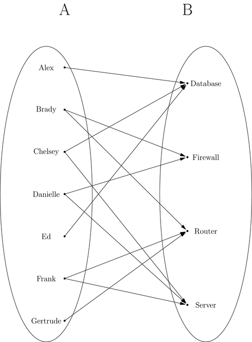
It should be apparent from Example 5.5.4 that arrow diagrams can look cluttered. Even with the visual clutter (which can be managed), arrow diagrams prove very useful, as we’ll see in the next chapter.
Tree Diagrams
One shortcoming with the previous methods is that they do not easily accommodate Cartesian Products with three or more sets.
Tree diagrams easily accommodate more than two sets in a Cartesian Product. However, depending on how many elements are in the sets, tree diagrams can become quite unwieldy.
A tree diagram is usually constructed starting from the left and progressing to the right. We start with a single dot, called the root of the tree. From this root, lines emanate to each of the elements in the first set listed in the Cartesian Product. Then, from each element in that first set, a line is extended to each of the elements from the second set listed in the Cartesian Product. However, each element of the first set gets its own copy of the elements in the second. Along each branch of the tree, we write the n-tuple containing all elements up to that branch in the tree. This process is repeated for each subsequent set in the Cartesian Product.
In a standard deck of playing cards, each card has a suit which can be one of
Spades (♠), Hearts (♥), Diamonds (♦), or Clubs (♣). Furthermore, each
card is colored either Red (R) or Black (B).
Also consider a coin, which when flipped, either results in Heads (H) or Tails
(T).
We capture these outcomes in the following sets.
\[
\begin{align*}
\text{Suit} &= \{\text{♠}, \text{♥}, \text{♦}, \text{♣}\} \\
\text{Color} &= \{\text{B}, \text{R}\} \\
\text{Flip} &= \{\text{H}, \text{T}\}
\end{align*}
\]
We construct the tree diagram for
$\text{Suit} \times \text{Color} \times \text{Flip}$ below:
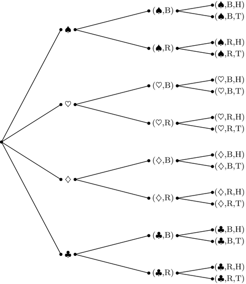
Notice in Example 5.5.5 that in the first level of the tree the elements are not enclosed in parentheses ( ). Since they are single elements, there is not much point in surrounding them, creating 1-tuples. At that point, we have not formed a Cartesian Product, so it’s unnecessary. Though in a sense, a single element could be considered a 1-tuple by itself. Either way, we intentionally do not enclose the first elements in ( ).
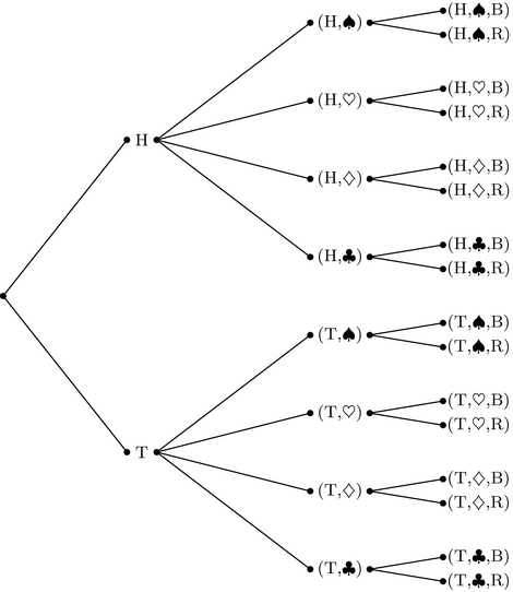
Remember that order matters when writing the sets in a Cartesian Product. As such, we expect the tree diagram representing the Cartesian Product to look different based on how the sets are ordered.
Reconsider the sets from Example 5.5.5. A tree diagram for
$\text{Flip} \times \text{Suit} \times \text{Color}$ would look like this:
To represent a relation, we simply remove any branches that yield n-tuples that are not in the relation. The act of removing such branches is sometimes called pruning in keeping with the arbor theme.
Reconsider the tree diagram from Example 5.5.5 drawn in a different style:
Notice that in the second level with the ordered pairs that ♠ is being paired up with the color red. We also see that ♥ is being paired up with the color black. However, in a normal deck of cards, those suits are not those colors.
To make an authentic deck of cards, lets consider the following relation:
$$\mathcal{R} = \{(\text{s}, \text{c}, \text{f})\ |\ \bigl[(\text{s} = ♠ \lor ♣) \land (\text{c} = B)\bigr] \lor \bigl[(\text{s} = ♥ \lor ♦) \land (\text{c} = R)\bigr] \}$$This relation says that if the card is in the relation and has a suit of spades or clubs, that would imply the card’s color is black. Similarly, if a card in the relation has a suit of either hearts or diamonds, that would imply that the card’s color is red.
Let’s put a slash through each branch that yields ordered pairs not in $\mathcal{R}$.
We don’t need to prune any sub-branches because they are considered pruned if their ancestor branches are pruned. We could go one step further and simply redraw the tree diagram without any of the pruned branches.
With less branches, we could make an equivalent tree diagram that is a little more compact:
Note that we don’t necessarily have to construct the tree for the entire Cartesian Product, and then prune branches to get the tree diagram for the desired relation. We could instead preemptively prune to prevent the tree from growing too large in the first place.
Reconsider the Cartesian Product $\text{Flip} \times \text{Suit} \times \text{Color}$ from Example 5.5.6. Suppose we impose the following conditions:
- Heads can’t pair up with Hearts
- Tails can only pair up with Diamonds
Of course, just like with Example 5.5.7, we would like to exclude any ordered triples that yield improperly colored cards. Instead of constructing the tree for the entire Cartesian Product, let’s just draw what we need: